Link Prediction using Similarity Measures

01Pre-requisite

02Preamble

This is going to be the last part of our three-part series on link predictions in social networks. In the first part, I showed you how to visualize a huge complex network of the size of Facebook. In the second part, I showed you how the “People you may know” type of features are implemented in such networks using Node2Vec. In this third and final part, I will show you how to enhance this link prediction using similarity measures.

03Introduction

For training our network model for predictions, we used Node2Vec earlier. The Node2Vec generates features internally and thus we do not have any control on what features it generates and how are they generated? By using the different similarity measures algorithms, you will get the control on features selection and thus optimize your algorithm for better predictions. To understand what is a similarity measure, I will first describe a little of theory on each of the measures that we will use in this tutorial. The measures we are going to use are:

• Common Neighbors
• Jaccard Coefficient
• Resource Allocation Index
• Adamic Adar Index
• Preferential Attachment
• Community Common Neighbors
• Community Resource Allocation Index

04Similarity Measures

A similarity measure determines the similarity between the two neighbouring nodes and thus helps in predicting the likelihood of their connection in the future.

05Common Neighbors

The common-neighbors predictor captures the notion that a common friend may introduce two strangers to each other. It tells us about the total number of common friends a pair of nodes have.

06Jaccard Coefficient

It is a similarity metric that is commonly used in information retrieval. It measures the probability that both x and y have a feature f, where f is a randomly selected feature of either x or y. If we take “features” here to be a determining factor of being neighbors, then this measure captures intuitively appealing notion that the proportion of the coauthors of x who have also worked with y (and vice versa) is a good measure of the similarity between x and y. Mathematically, it is expressed as:

The Jaccard coefficient of nodes X and Y is;

Do not worry, even if you do not understand these mathematical expressions. We have ready-to-use implementations for the same, and you will learn to use them soon.

07Resource Allocation Index

Resource Allocation Index is obtained by calculating the average score for each cluster and then by averaging those scores, it is simply the average of the common neighbors score. Mathematically, it is expressed as:

The Resources Allocation index of nodes X and Y is;

08Adamic Adar Index

This measure refines the simple counting of common features by weighing rarer features more heavily. The Adamic/Adar predictor formalizes the intuitive notion that rare features are more telling; documents that share the phrase “for example” are probably less similar than documents that share the phrase “clustering coefficient.”

According to the mathematical expression below, the more friends ‘u’ has, the lower score it will be assigned to. Thus, the common neighbour of a pair of nodes with few neighbors contributes more to the Adamic/Adar score (AA) value than this with many relationships. In a real-world social network, we interpret it as follows: if a common acquaintance of two people has more friends, then it is less likely that he will introduce the two people to each other than when he has only few friends.

The Adamic-Adar index of nodes X and Y is;

09Preferential Attachment

One well-known concept in social networks is that users with many friends create more connections in the future. This is like in some social networks, such as financial markets, the rich get richer. We estimate how “rich” our two vertices are by calculating the multiplication between the number of friends (|N(x)|, number of friends x has, and |N (y) |) or followers each vertex has. We may note that the similarity index does not require any node neighbor information; therefore, this similarity index has the lowest computational complexity. Mathematically, the preferential attachment score of nodes X and Y is expressed as:

10Community Common Neighbors

It is the measure of the number of common neighbors a node has, when all the neighbor nodes and the given node are under the same community. We can say two nodes to belong to the same community if they both have the same given feature, like for example, city or age group or school, etc.

The common Neighbor Soundarajan-Hopcroft score of nodes Y and Y is:

11Community Resource Allocation Index

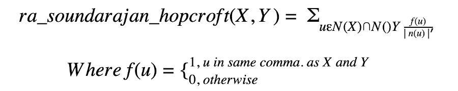
This measure computes the resource allocation index of all node pairs with common node pairs and gives a bonus for node pairs in the same community.

The Resource Allocation Soundarajan-Hopcroft score of nodes Y and Y is:

These are all the similarity measures that we will use for determining features, So let’s start.

12Creating Project

Create a new Colab project and rename it to Similarity Measures.

13Import Libraries

As usual we first import the required libraries.

import random
from tqdm import tqdm
import networkx as nx
from zipfile import ZipFile
import pandas as pd
import numpy as np
import matplotlib.pyplot as plt
import seaborn as sns
%matplotlib inline
 
from warnings import simplefilter
from sklearn.exceptions import ConvergenceWarning
simplefilter("ignore", category=ConvergenceWarning)

14Downloading Data

We download the master data file. This zip contains all files for all the three parts. But we only require the graph G and dataframe df1 here.

!wget https://github.com/abcom-mltutorials/Facebook-Social-Network-Analysis/archive/master.zip -P "/content"
ZipFile("/content/master.zip").extractall("/content/")

Next, retrieve the graph G and df1 dataframe from the part II (Node2Vec) of this series.

G = nx.read_gpickle('/content/Facebook-Social-Network-Analysis-master/Graph.pickle')
df1 = pd.read_csv('/content/Facebook-Social-Network-Analysis-master/df1.csv', index_col=[0])

To recapitulate, print the network information

#printing information about the graph
print(nx.info(G))

The output is shown below:

Name: Facebook SNA Graph
Type: Graph
Number of nodes: 1295
Number of edges: 18321
Average degree:  28.2950

Print the data frame.

#printing the df1 dataframe
df1

The output is shown below:

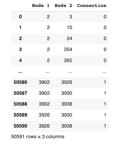
The dataframe shows the connection probability between the two nodes.

15Generate Features

We will create a copy of the df1 dataframe, which contains the positive and negative samples, i.e. the future connections. We will change this copy for further processing.

#making a copy of the original dataframe
df_2 = df1.copy()
 
#sorting according to the nodes
df_2.sort_values(['Node 1', 'Node 2'], inplace=True)
 
#getting the two nodes in a row in a tuple, i.e (Node 1, Node 2) and adding then to a new Edges column
edges = [(df1.iloc[i,0],df1.iloc[i,1]) for i in range(df1.shape[0])]
df_2['Edges'] = edges
 
#dropping the Node 1 and Node 2 columns and setting the Edges column as index
df_2.drop(columns=df_2.columns[:2], inplace=True)
df_2.set_index('Edges', inplace=True)
 
df_2.head()

The output is shown below:

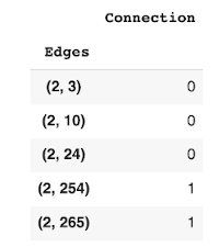
The new dataframe now lists out edges between the two nodes and shows the probability of a connection between them.

We are now ready to process our data and apply the different similarity measures that I discussed earlier. Fortunately for us, the nx library provides the ready-to-use implementations of these similarity measures.

16Common Neighbors

We generate the common neighbours using the following statement and add it to the df_2 dataframe as a column.

df_2['Common_Neigh'] = [len(list(nx.common_neighbors(G, e[0],e[1]))) for e in df_2.index]

17Jaccard Coefficient

We will first find the Jaccard Coefficients of the edges and put them into a new dataframe according to their edges and then we will merge the new dataframe with our original dataframe.

The jaccard coefficient is computed using the built-in function of nx library. We store the computed coefficient in a new data frame - df_3. We then merge the two frames to give us the revised df_2 containing both common neighbours and jaccard.

#creating a new temporary dataframe for storing the similarity measure values
df_3 = pd.DataFrame()
 
#finding jaccard coefficients
jaccard = list(nx.jaccard_coefficient(G, list(df_2.index)))
 
#storing the values in the new dataframe and setting the index as edges
df_3['Jaccard_Coef'] = [i[2] for i in jaccard]
df_3['Edges'] = [(i[0],i[1]) for i in jaccard]
df_3.set_index('Edges', inplace=True)
 
#merging the new dataframe with our previous 'df2' dataframe
df_2 = df_2.join(df_3, how='inner')

18Resource Allocation Index

We follow the procedure as earlier to compute the resource allocation index and merge it into our df_2 array.

df_3 = pd.DataFrame()
 
#finding resource allocation index
resource_alloc = list(nx.resource_allocation_index(G, list(df_2.index)))
 
#storing the values in a new dataframe and setting the index as edges
df_3['Resource_Alloc'] = [i[2] for i in resource_alloc]
df_3['index'] = [(i[0],i[1]) for i in resource_alloc]
df_3.set_index('index', inplace=True)
 
#merging the new dataframe with our previous 'df2' dataframe
df_2 = df_2.join(df_3, how='inner')

19Adamic Adar Index

We compute this index using the built-in adamic_adar_index function and add it to the df_2 dataframe as earlier.

df_3 = pd.DataFrame()
 
#finding adamic adar index
adamic_adar = list(nx.adamic_adar_index(G, list(df_2.index)))
 
#storing the values in a new dataframe and setting the index as edges
df_3['Adamic_Adar'] = [i[2] for i in adamic_adar]
df_3['index'] = [(i[0],i[1]) for i in adamic_adar]
df_3.set_index('index', inplace=True)
 
#merging the new dataframe with our previous 'df2' dataframe
df_2 = df_2.join(df_3, how='inner')

20Preferential Attachment

We compute the preferential attachment using the preferential_attachment method and add it to the df_2 frame.

df_3 = pd.DataFrame()
 
#finding preferential attachment
preferential_attach = list(nx.preferential_attachment(G, list(df_2.index)))
 
#storing the values in a new dataframe and setting the index as edges
df_3['Preferential_Attach'] = [i[2] for i in preferential_attach]
df_3['index'] = [(i[0],i[1]) for i in preferential_attach]
df_3.set_index('index', inplace=True)
 
#merging the new dataframe with our previous 'df2' dataframe
df_2 = df_2.join(df_3, how='inner')

21Community Common Neighbors

The code for computing the community common neighbors and adding it to df_2 is given below:

df_3 = pd.DataFrame()
 
#finding community common neighbors, community is the 'location;id'
community_common_neigh = list(nx.cn_soundarajan_hopcroft(G,list(df_2.index), community='location;id'))
 
#storing the values in a new dataframe and setting the index as edges
df_3['Community_Comnon_Neigh'] = [i[2] for i in community_common_neigh]
df_3['index'] = [(i[0],i[1]) for i in community_common_neigh]
df_3.set_index('index', inplace=True)
 
#merging the new dataframe with our previous 'df2' dataframe
df_2 = df_2.join(df_3, how='inner')

22Community Resource Allocation Index

The community for this index is the location:id. We commute this index and store it in df_1 using the following code:

df_3 = pd.DataFrame()
 
#finding community resource allocation index, community is the 'location;id'
community_resource_alloc = list(nx.ra_index_soundarajan_hopcroft(G,list(df_2.index), community='location;id'))
 
#storing the values in a new dataframe and setting the index as edges
df_3['Community_Resource_Alloc'] = [i[2] for i in community_resource_alloc]
df_3['index'] = [(i[0],i[1]) for i in community_resource_alloc]
df_3.set_index('index', inplace=True)
 
#merging the new dataframe with our previous 'df2' dataframe
df_2 = df_2.join(df_3, how='inner')

As we have not computed all our similarity measures and stored them in df_2, let us print a few records to see the results.

23Printing Similarity Measures Values

We print the few records of df_2 by calling its head method.

df_2.head()

The output is as shown below:

You may examine the various columns to understand the similarity between different nodes as predicted by different measures.

24Understanding Correlation

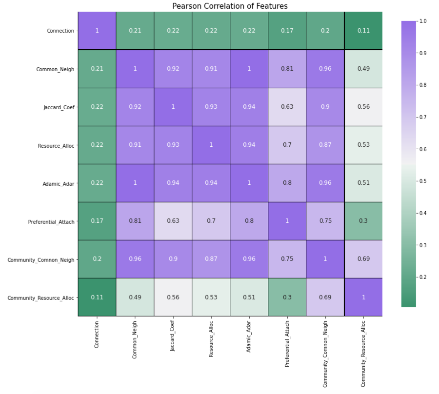
We will now do a correlation matrix plot to understand the relationship between the different measures. We generate the plot using the following code:

_ , ax = plt.subplots(figsize =(14, 12))
 
#setting the colormap
colormap = sns.diverging_palette(150, 275, s=80, l=55, n=9, as_cmap = True)
 
#creating the heatmap
_ = sns.heatmap(df_2.corr(), cmap = colormap, square=True, cbar_kws={'shrink':.9 }, ax=ax, annot=True,
                                                    linewidths=0.1,vmax=1.0, linecolor='black', annot_kws={'fontsize':12 })
  
#adding title
plt.title('Pearson Correlation of Features', y=1.05, size=15)

The output is shown below:

Now, we have the dataset containing all the desired similarity measures. We will now apply different machine learning algorithms on this dataset to get the best results for similarity measures.

25Creating Model

Import the necessary libraries:

from sklearn.ensemble import RandomForestClassifier
from sklearn.ensemble import GradientBoostingClassifier
from sklearn.neural_network import MLPClassifier
from sklearn.model_selection import train_test_split
from sklearn.model_selection import GridSearchCV
from sklearn.metrics import accuracy_score, precision_score, recall_score, f1_score, auc, roc_curve, roc_auc_score,confusion_matrix

Set the features:

#features    
X = df_2.iloc[:,1:]

Set the target:

#target
y = df_2['Connection']

Create train/test datasets:

X_train, X_test, y_train, y_test = train_test_split(X, y, random_state = 0)

Scale the dataset:

from sklearn.preprocessing import MinMaxScaler
scaler = MinMaxScaler()
 
#this will be used only for MLP Classifier
X_train_scaled = scaler.fit_transform(X_train)
X_test_scaled = scaler.transform(X_test)

26Search Best Algorithm

Like in Part II of this series, we will use GridSearchCV to test the three classifier algorithms, viz. Random Forest, Gradient Boost, and MLP.

27Random Forest

Applying Random Forest, using GridSearchCV, on X_train and y_train and testing the model’s accuracy score using X_test and y_test.

#classifier
clf1 = RandomForestClassifier()
 
#parameters
param = {'n_estimators' : [10,50,100], 'max_depth' : [5,10,15]}
 
#model
grid_clf_acc1 = GridSearchCV(clf1, param_grid = param)
 
#training the model
grid_clf_acc1.fit(X_train, y_train)
 
print('Grid best parameter (max. accuracy): ', grid_clf_acc1.best_params_)
print('Grid best score (accuracy): ', grid_clf_acc1.best_score_)
 
# alternative metric to optimize over grid parameters: AUC
grid_clf_auc1 = GridSearchCV(clf1, param_grid = param, scoring = 'roc_auc')
grid_clf_auc1.fit(X_train, y_train)
predict_proba = grid_clf_auc1.predict_proba(X_test)[:,1]
 
print('Test set AUC: ', roc_auc_score(y_test, predict_proba))
print('Grid best parameter (max. AUC): ', grid_clf_auc1.best_params_)
print('Grid best score (AUC): ', grid_clf_auc1.best_score_)

The output is as follows:

Grid best parameter (max. accuracy):  {'max_depth': 10, 'n_estimators': 200}
Grid best score (accuracy):  0.6819969189376212
Test set AUC:  0.6272261793061837
Grid best parameter (max. AUC):  {'max_depth': 5, 'n_estimators': 200}
Grid best score (AUC):  0.6480656778572059

28Gradient Boost

Applying Gradient Boost, using GridSearchCV, on X_train and y_train and testing the model’s accuracy score using X_test and y_test.

#classifier
clf2 = GradientBoostingClassifier()
 
#parameters
param = {'learning_rate' : [.05,.1]}
 
#model
grid_clf_acc2 = GridSearchCV(clf2, param_grid = param)
 
#training the model
grid_clf_acc2.fit(X_train, y_train)
 
print('Grid best parameter (max. accuracy): ', grid_clf_acc2.best_params_)
print('Grid best score (accuracy): ', grid_clf_acc2.best_score_)
 
# alternative metric to optimize over grid parameters: AUC
grid_clf_auc2 = GridSearchCV(clf2, param_grid = param, scoring = 'roc_auc')
grid_clf_auc2.fit(X_train, y_train)
predict_proba = grid_clf_auc2.predict_proba(X_test)[:,1]
 
print('Test set AUC: ', roc_auc_score(y_test, predict_proba))
print('Grid best parameter (max. AUC): ', grid_clf_auc2.best_params_)
print('Grid best score (AUC): ', grid_clf_auc2.best_score_)

The output is as follows:

Grid best parameter (max. accuracy):  {'learning_rate': 0.1}
Grid best score (accuracy):  0.6798357783193818
Test set AUC:  0.6455543580803677
Grid best parameter (max. AUC):  {'learning_rate': 0.1}
Grid best score (AUC):  0.6481376190393812

29MLP Classifier (A Neural Network Classifier)

Applying MLP Classifier, using GridSearchCV, on X_train and y_train and testing the model’s accuracy score using X_test and y_test.

#classifier
clf3 = MLPClassifier(max_iter=1000)
 
#scaling training and test sets
from sklearn.preprocessing import MinMaxScaler
scaler = MinMaxScaler()
X_train_scaled = scaler.fit_transform(X_train)
X_test_scaled = scaler.transform(X_test)
 
#parameters
param = {'hidden_layer_sizes' : [10,100,[10,10]], 'activation' : ['tanh','relu'], 'solver' : ['adam','lbfgs']}
 
#model
grid_clf_acc3 = GridSearchCV(clf3, param_grid = param)
 
#training the model
grid_clf_acc3.fit(X_train_scaled, y_train)
 
print('Grid best parameter (max. accuracy): ', grid_clf_acc3.best_params_)
print('Grid best score (accuracy): ', grid_clf_acc3.best_score_)
 
# alternative metric to optimize over grid parameters: AUC
grid_clf_auc3 = GridSearchCV(clf3, param_grid = param, scoring = 'roc_auc')
grid_clf_auc3.fit(X_train_scaled, y_train)
predict_proba = grid_clf_auc3.predict_proba(X_test_scaled)[:,1]
 
print('Test set AUC: ', roc_auc_score(y_test, predict_proba))
print('Grid best parameter (max. AUC): ', grid_clf_auc3.best_params_)
print('Grid best score (AUC): ', grid_clf_auc3.best_score_)

The output is shown below:

Grid best parameter (max. accuracy):  {'activation': 'tanh', 'hidden_layer_sizes': [10, 10], 'solver': 'lbfgs'}
Grid best score (accuracy):  0.6795195276463806
Test set AUC:  0.6437530783683811
Grid best parameter (max. AUC):  {'activation': 'relu', 'hidden_layer_sizes': 100, 'solver': 'lbfgs'}
Grid best score (AUC):  0.6492073396352226

30Summarizing

I have tabulated the results of the above training, which is shown here.

                                        Random Forest	Gradient Boost	MLP Classifier
Best Score (accuracy)	0.6819	        0.6798	        0.6795
Best Score AUC	            0.6480	        0.6481	        0.6492
Test Set AUC	                0.6272	        0.6455	        0.6437

Random Forest classifier outperforms the other two in terms of accuracy. So, we will use this one for inference.

31Inference

We perform the predictions on our test dataset by calling the predict method:

#getting predictions of out test data
pred = grid_clf_acc1.predict(X_test_scaled)

We examine the first five predictions.

pred[:5]

The output is as follows:

array([0, 0, 0, 0, 0])

The output indicates that the likelihood of connection between the first five edges is very low.

32Accuracy Score

Print the accuracy score

accuracy_score(pred,y_test)

It gives the following output:

0.676944971537002

As we can see that our accuracy is quite lower than the previous method. This is because our dataset is highly imbalanced, i.e. having several nodes with no edge between them. Having a more balanced dataset would improve the results. Again, including more factors to find out and decide why two nodes are connected can help improve the score. Like for example, we have used only two factors for our model, namely location and education school, you could mix in other factors available in the dataset to enhance the model’s inference.

33Confusion Matrix

Generate the confusion matrix:

confusion_matrix(pred,y_test)

The output is as follows:

array([[7288, 3048],
       [1038, 1274]])

The confusion matrix shows that 8562 values (7288 (True Positive) + 1274 (True Negative)) are correct and 4086 values (3048 (False Positive) + 1038 (False Negative)) are incorrect.

34The ROC_AUC Score and ROC Curve

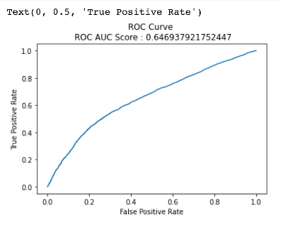
Now, let’s find the ROC_AUC Score and plot the ROC Curve in the similar fashion as we had done in the previous part (part II).

predict_proba = grid_clf_acc1.predict_proba(X_test_scaled)[:,1]
 
false_positive_rate,true_positive_rate,_ = roc_curve(y_test, predict_proba)
roc_auc_score = auc(false_positive_rate,true_positive_rate)
 
#plotting
plt.plot(false_positive_rate,true_positive_rate)
plt.title(f'ROC Curve 
 ROC AUC Score : {roc_auc_score}')
plt.xlabel('False Positive Rate')
plt.ylabel('True Positive Rate')

The output is shown below:

35Demonstration

Now, we come to a real use-case of our entire analysis so far. We will find the probability of two nodes forming an edge.

First let’s look at our dataframe.

df_2.head()

Let’s choose nodes 2 and 24. These nodes do not have an edge between them denoted by ‘0’ in the Connection column.

We need to get the features of the node pair (2,24) from the ‘X’ array, containing all the node pair features, which we had created earlier, and we need to find the index of this node pair features in the X_train dataframe.

Note : Features for node pairs (2, 24) are in X_train but some node pair features will be in X_test, since X has been divided into X_train and X_test.

# from the above dataframe let's choose the nodes 2 and 24
# node pair (2,24) is at index 2, hence let's print it's features
 
print(f' ({df_2.index[2][0]},{df_2.index[2][1]}) node pair features : {X.iloc[2,:]}')
 
# its position in X_train
print(f'Index of ({df_2.index[2][0]},{df_2.index[2][1]}) node pair in X_train : {np.where(X_train.index == X.index[2])[0][0]}')

This is the output:

(2,24) node pair features : Common_Neigh                 0.0
Jaccard_Coef                 0.0
Resource_Alloc               0.0
Adamic_Adar                  0.0
Preferential_Attach         27.0
Community_Comnon_Neigh       0.0
Community_Resource_Alloc     0.0
Name: (2, 24), dtype: float64
Index of (2,24) node pair in X_train : 22897

You can see that the index for node pair (2,24) in X_train is 22897. We can see that all the similarity measures for this node pair is 0, and only the similarity measure of Preferential attachment is 27.

Now we are going to predict the probability of an edge forming between these two nodes in the future, using the predict_proba function. We will be using X_train_scaled since we have used the scaled version to train our model. X_train and X_train_scaled have values at the same indices.

predict_proba = grid_clf_acc1.predict_proba(X_train_scaled[np.where(X_train.index == X.index[2])[0][0]].reshape(1,-1))[:,1]
 
print(f'Probability of nodes {df_2.index[2][0]} and {df_2.index[2][1]} to form a link is : {float(predict_proba)*100 : .2f}%')

The output is as follows:

Probability of nodes 2 and 24 to form a link is :  13.18%

36Conclusion

The second method for link prediction, creating features out of similarity measures, does so poorly only because we have used a highly imbalanced dataset, i.e. large number of ‘0’ values in the ‘Connection’ column and less of ‘1’ values. If we had used a more balanced dataset, then it would have resulted in more positive samples or less negative samples (regarding the confusion matrix), and hence the model would have provided a much better score. But in reality, datasets are highly imbalanced.

37Summary

In this part of the project you learnt how one can make link predictions by using the features generated using similarity measures. You also learnt what similarity measures are and got an idea how to use them. Next the similarity measures for the node pairs in our graph were generated, and we used them as the features for your model. We applied GridSearch on three ML algorithms, Random Forest, Gradient Boost and MLP Classifier, using two scoring methods, accuracy and roc_auc, to find out the best model. We concluded that Random Forest gives us the best accuracy, and hence we use that as our final model.

This was the last part of the project. Go on, try to implement this on your own!