Mall Customer Segmentation

01

Have you ever wondered how Burger King or Pizza Hut comes up with an on-the-spot offer when you visit a Mall? Certainly, your mobile location is tracked and if you are a Pizza or Burger lover as shown by your past eating history, you get invited for such offers. These days, most malls track customers and their purchase habits and provide this information to the shop owners in the mall. We investigate gathered data using market basket analysis to group customers into different segments according to their preferences. In this tutorial you will learn some machine learning techniques to perform such analysis and develop a model using K-Means clustering to create customer segments.

Let us start by creating a project.

02Customer Segmentation

Any machine learning project requires a dataset for training the model. I have picked up the data from Kaggle for this purpose. The database is small, but will surely help you understand the various EDA (Exploratory Data Analysis) techniques and using a K-Means clustering algorithm for segmentation. I have made the dataset available on our GitHub for easy access to this project.

You will use Google Colab for creating the model.

03Creating Project

Create a new Colab project and rename it to MallCustomerSegmentation. In the project, first import the required libraries.

import numpy as np
import pandas as pd
import matplotlib.pyplot as plt
import seaborn as sns
import plotly as py
import plotly.graph_objs as go
from sklearn.cluster import KMeans
import warnings
warnings.filterwarnings("ignore")

04Downloading Dataset

Download the dataset using wget command. The wget downloads the data straight into your Google drive making it available into your Colab project.

!wget https://raw.githubusercontent.com/abcom-mltutorials/mall/main/Mall_Customers.csv

Load the downloaded .csv file into pandas dataframe:

data = pd.read_csv('Mall_Customers.csv')
data.head()

Examine few records

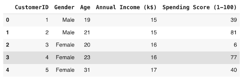
Check the dataset size by calling the shape method.

data.shape

Output:

(200, 5)

As you can see, there are only 200 data points and only 5 columns. The K-Means algorithm works beautifully even on such small datasets. You will see this soon.

We will now change the names of few columns for our convenience:

data = data.rename(columns={'Annual Income (k$)': 'Annual_income', 'Spending Score (1-100)': 'Spending_score'})

Check the detailed summary of the dataset by calling the info method

data.info()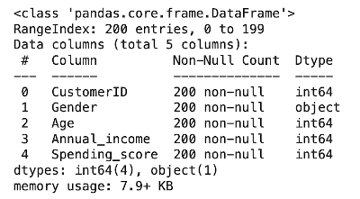

Here we get the information about the number of rows, number of columns, data types and number of null values in each column.

We analyze the data distribution by calling the describe method:

data.describe()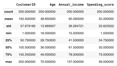

It shows the descriptive statistics like mean, median, mode, percentiles, min, max and standard deviation of the columns of the dataset.

05Data Cleaning

Checking for the null values:

data.isnull().sum()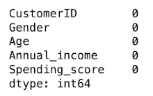

Replacing categorical values with numerics:

data.Gender.replace('Male', 0, inplace=True)
data.Gender.replace('Female', 1, inplace=True)
data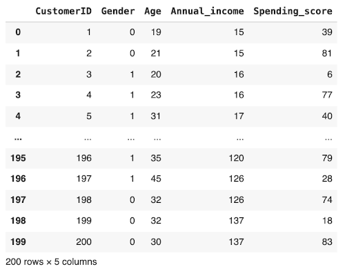

Our data preprocessing is now completed. We now proceed to the various EDA techniques.

06Data Visualization

To explore and understand the dataset, we generate the various plots. We begin by plotting the gender distribution.

07Gender Distribution

We will check the distribution of male/female customers in our dataset by creating a pie chart. Certainly we would like to know if the female shoppers outnumber the males? We do this plot using the following code:

labels = ['Female', 'Male']
size = data['Gender'].value_counts()
colors = ['yellow', 'salmon']
explode = [0, 0.1]

plt.rcParams['figure.figsize'] = (9, 9)
plt.pie(size, colors = colors, explode = explode, labels = labels, shadow = True, autopct = '%.2f%%')
plt.title('Gender', fontsize = 20)
plt.axis('off')
plt.legend()
plt.show()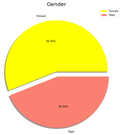

From the chart, we can see that 56% of our customers are female and the rest are male.

Next, we examine the correlation between the variables.

08Variable Correlations

We will examine the relationship between Age, Annual_income and Spending _score by generating the pairplots. We do this using the following statement:

sns.pairplot(data, vars=["Age", "Annual_income", "Spending_score"],  kind ="reg", hue = "Gender", markers = ['o','D'])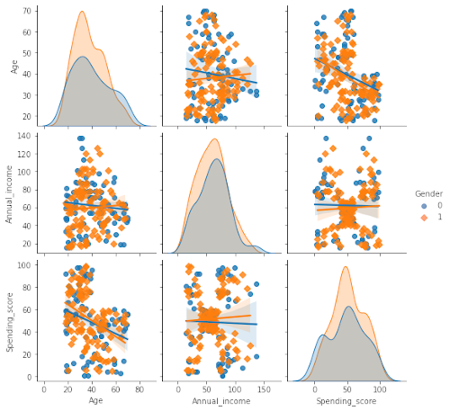

From these plots, we easily observe the relation between the different variables in the dataset. Along the diagonal, observe the histograms. We clearly see that the women are always more prominent in shopping than men regarding their age, annual income and spending score. Study other plots to see the relationship between the other variables marked in different colors for men and women.

Now, we will prepare the dataset for K-Means clustering.

09Preparing Data for Modeling

Extract the CustomerID and Gender into another variable - note that these two columns are not the predictors or features for clustering.

data_id = data[['CustomerID','Gender']].copy()

Create a predictor list with the rest of the columns.

data_predictor = data.drop(['CustomerID', 'Gender'], axis=1)

10K-Means Clustering

Now, we are all set for clustering. We first need to decide on the number of clusters we want to create in our dataset. We do so by using the Silhouette and Elbow methods.

11Silhouette Analysis

The average silhouette approach measures the quality of clustering. It determines how well each object lies within its cluster. An above average silhouette width shows a good clustering. The average silhouette method computes the average silhouette of observations for different values of K.

#Importing Silhouette score module
from sklearn.metrics import silhouette_score
    
for num_clusters in range(2,10):
    # Instantiate k-means
    kmeans = KMeans(n_clusters=num_clusters, max_iter=50, random_state=50)
    # Fit the
    kmeans.fit(data_predictor)
    # Labels of each cluster point
    cluster_labels = kmeans.labels_
    
    silhoutte_avg = silhouette_score(data_predictor, cluster_labels)
    print("For n_clusters={0} the silhouette score={1}".format(num_clusters, silhoutte_avg))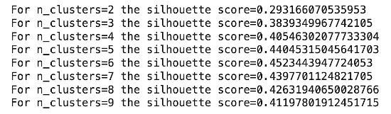

We see that the highest value of silhouette score exists for k = 5 & 6. Therefore, we conclude that the optimal number of clusters for the data can be 5 or 6.

12Elbow Method

The elbow method is used to determine the optimal number of clusters in K-Means clustering. The elbow method plots the value of the cost function produced by different values of K and one should choose several clusters so that adding another cluster doesn’t give much better modeling of the data. We will use WCSS (Within Cluster Sum of Squares) as our cost function.WCSS is the sum of squares of the distances of each data point in all clusters to their respective centroids.

We calculate WCSS using the following formula:

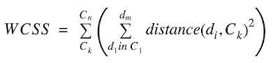
Where, C is the cluster centroids and d is the data point in each Cluster.

The code below plots the inertia for various cluster values.

ssd = []
for k in range(2,10):
    kmeans = KMeans(n_clusters = k).fit(data_predictor)
    ssd.append([k, kmeans.inertia_])
plt.plot(pd.DataFrame(ssd)[0], pd.DataFrame(ssd)[1])
plt.title('The Elbow Method', fontsize = 20)
plt.xlabel('Number of Clusters')
plt.ylabel('Inertia')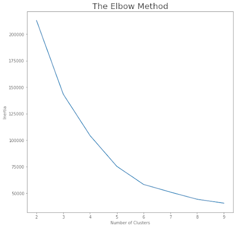

Imagine this curve as an arm stretched out. We notice an elbow at a cluster value of 5. This is the optimal number of clusters found by the Elbow method. We will use this value for clustering our data.

13Clustering

Instantiate the K-Means with K =5:

kmeans = KMeans(n_clusters=5, max_iter=50, random_state=50)

Fit the model:

kmeans.fit(data_predictor)

Now, print the labels for each data point.

kmeans.labels_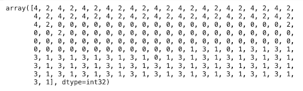

The above array output shows which customer belongs to which cluster. Note that each data point gets a label between 0 through 4 showing the cluster to which they are classified.

Now, I will show you a few visualizations on the results.

14Visualization

Copy data_predictor data frame to data_kmeans:

data_kmeans = data_predictor.copy()

Add the cluster labels to the dataframe to show which customer belongs to which group of cluster. Add the array output in the data frame as a column named as ClusterID.

data_kmeans['ClusterID'] = kmeans.labels_
data_kmeans.head()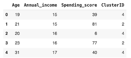

Get the count of customers into each cluster.

data_kmeans['ClusterID'].value_counts()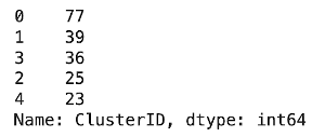

Concat data_id and data_kmeans, so as to include CustomerID and Gender that we have copied previously for further visualization.

data_kmeans = pd.concat([data_id, data_kmeans], axis=1)
data_kmeans.head()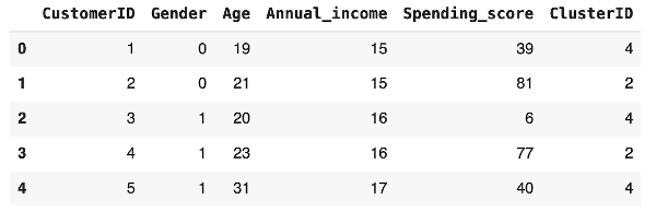

Plot the chart of number of customers in each cluster using the following code:

plt.figure(figsize=(12,7))
axis = sns.barplot(x=np.arange(0,5,1),y=data_kmeans.groupby(['ClusterID']).count()['CustomerID'].values)
x=axis.set_xlabel("Cluster Number")
x=axis.set_ylabel("Number of Customers")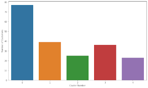

We can see that Cluster-0 has 77, Cluster-1 has 39, Cluster-2 has 25, Cluster-3 has 36 and Cluster-4 has 23 customers.

Now, we have clusters assigned to each of our customers. We will now profile these customers based on their features.

15Customer Profiling

Merge the original data with cluster id:

data_clustered = pd.merge(data, data_kmeans[['CustomerID','ClusterID']], on='CustomerID')
data_clustered.head()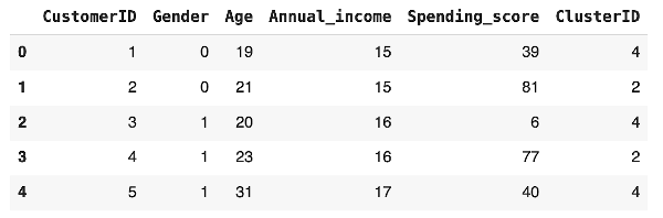

We will try to find the relationship between age and the annual income for customers in different clusters.

16Age and Annual Income

Generate a plot to understand the correlation between age and annual income using the following code:

sns.scatterplot(x = "Age", y = "Annual_income", data = data_clustered, hue = "Gender")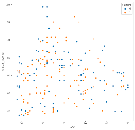

From the plot, you can see that customers in the age group 30 through 50 have better annual income than the younger age group and the older people. The red and blue dots show the distribution of men and women in each group.

We will now try to understand the relationship between spending score and income for both men and women.

17Spending Score and Annual Income

The plot is generated using the following code:

sns.scatterplot(x = "Annual_income", y = "Spending_score", data = data_clustered, hue = "Gender")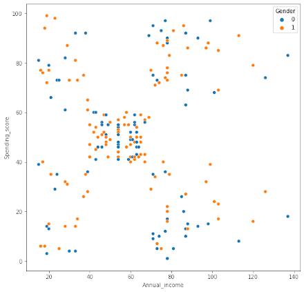

From the output, you can see that the customers having an annual income between 50 to 60 have reasonable spending habits, while some customers having either low or high income are better spenders.

Next, we will look at the relationship between spending score and age.

18Age and Spending Score

The plot is generated using following code:

sns.scatterplot(x = "Age", y = "Spending_score", data = data_clustered, hue = "Gender")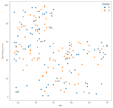

As you can see customers having age lower than 40, that is the younger people are better spenders in malls. Malls target the young people with attractive offers on Games Parlors, Tech Stores, Foods and Beverages.

We will now do an analysis of the clusters based on the customer features.

19Cluster Analysis

Check the mean values of Age, Annual_income and Spending_score for each cluster:

data_clustered[['Age', 'Annual_income', 'Spending_score', 'ClusterID']].groupby('ClusterID').mean()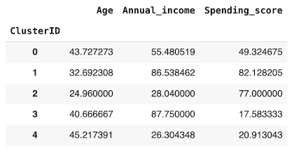

The table shows the average age, income and spending score for each of the clusters. You may visualize this distribution by generating a bar chart.

data_clustered[['Age', 'Annual_income', 'Spending_score', 'ClusterID']].groupby('ClusterID').mean().plot(kind='bar',log=True,figsize = (8,6))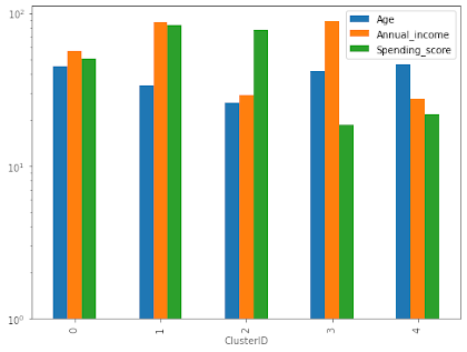

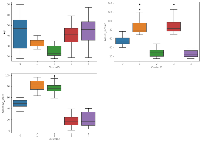
Some of you may prefer visualization of these parameters using box plots, which are drawn using following code:

var_analysis = ['Age', 'Annual_income', 'Spending_score']
plt.figure(figsize = (14,10))
for i in enumerate(var_analysis):
    plt.subplot(2,2,i[0]+1)
    sns.boxplot(x= 'ClusterID', y = i[1], data = data_clustered)

This is the output:

20Clustering

In clustering we will not be considering the gender factor anymore. The first primary reason we take this approach is because the difference between male and female in this data is not high and making a gender differentiation won’t provide any further information. The second and not least important reason is the fact that stores hardly ever target a specific gender anymore. Also, we do not want to interfere in the process of unsupervised learning. We will let the algorithm do its job and once it’s finished, we will analyze the results and extract conclusions and knowledge.

Training K-means with 5 clusters:

means_k = KMeans(n_clusters=5, random_state=0)
means_k.fit(data_predictor)
labels = means_k.labels_
centroids = means_k.cluster_centers_

As we can observe, the K-Means algorithm has already finished its work and now it’s time to plot the results we got by it so we can visualize the different clusters and analyze them.

213-D Visualization of Clusters

3-D Visualization of Clusters

trace1 = go.Scatter3d(
    x= data_predictor['Spending_score'],
    y= data_predictor['Annual_income'],
    z= data_predictor['Age'],
    mode='markers',
        marker=dict(
        color = labels,
        size= 10,
        line=dict(
            color= labels,
        ),
        opacity = 0.9
        )
    )
    layout = go.Layout(
    title= 'Clusters',
    scene = dict(
            xaxis = dict(title  = 'Spending_score'),
            yaxis = dict(title  = 'Annual_income'),
            zaxis = dict(title  = 'Age')
        )
    )
    fig = go.Figure(data=trace1, layout=layout)
    py.offline.iplot(fig)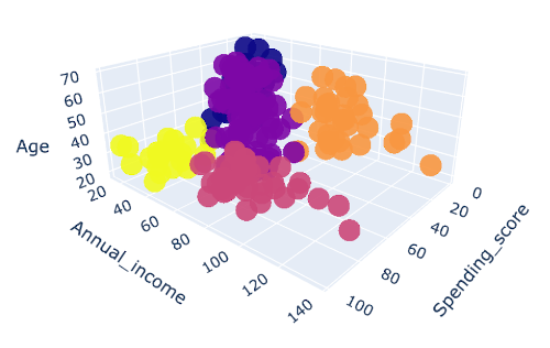

You should try the above visualization on your computer to see the 3-D effects.

The above plot displays firstly what a K-Means algorithm would yield using five clusters. We only fed three features to train our cluster model. This gives us enough data to put these features on a 3-D scale. Here, x-axis represents Spending_score, y-axis represents Annual_income and z-axis represents Age in the above graph.

After plotting the results got by K-Means on this 3-D graphic, it’s our job now to identify and describe the five clusters that have been created:

Yellow Cluster - The yellow cluster groups young people with moderate to low annual income who actually spend a lot

Purple Cluster - The purple cluster groups reasonably young people with pretty decent salaries who spend a lot

Pink Cluster - The pink cluster basically groups people of all ages whose salary isn't pretty high and their spending score is moderate

Orange Cluster - The orange cluster groups people who actually have pretty good salaries and barely spend money, their age usually lays between thirty and sixty years

Blue Cluster - The blue cluster groups whose salary is pretty low and spend a little money in stores, they are people of all ages.

22Summary

K-Means clustering is a powerful technique for classifying data into different categories. In this tutorial, you learned this technique for segmenting the customers in different categories. The customer segmentation allows you to understand the behavior of different customers and accordingly plan your marketing strategy. After we create the clusters, you learned how to understand the profiles of the customers in different segments. The technique that you learned here can easily be applied to other domains.