Live Tweets Disaster Analysis with BERT

01

Tweets probably use more erratic language than any other online text generation. People use all sorts of abbreviations, slangs, grammatically incorrect sentences, uncommon words, words not found in Oxford dictionary, and what not? At the same time, these tweets many times carry vital information that could be very useful to you even in saving somebody's precious life. You may still remember the doomed day of 9/11 (Terrorist attack on World Trade Center) or 26/11 (Mumbai terror attacks) when a single tweet might have alerted several to take a life-saving action.

Analyzing Twitter data for such vital information is a challenge due to the language people used while tweeting. You need to clean up the text to a great extent and also understand what they are trying to say, that is basically extracting vital information from the tweets. In this tutorial I will show you a few techniques of cleaning text data before we feed it to our neural network for Natural Language Understanding (NLU). We will use BERT ( Bidirectional Encoder Representations from Transformers) - a really powerful language representation model that has changed the NLP (Natural Language Processing) paradigm totally since last year.

“Handle them carefully, for words have more power than atom bombs.”

— Pearl Strachan Hurd

Our words say much more than we might think. If we pay good attention to words, we might extract some great valuable information. In this tutorial, we will use the power of BERT for information extraction.

02Project Description

‘You can have Data without information, but you cannot have information without data.’’

— Daniel Keys

Any Machine Learning application cannot be developed without a proper dataset. Fortunately, for our purpose, twitter data is available at Kaggle site for creating our ML model. The problem that we are trying to solve is essentially a text classification problem. For text classification, we need natural language understanding and that’s where we will use BERT for giving us insights of a given tweet. After you train the model on Kaggle dataset, I will show you how to classify the real time tweets for a practical use. For this, you will learn how to capture a live stream of tweets and classify them instantaneously.

03Creating a Project

Follow along and create a new Google Colab project and rename it to Live Tweet Analysis. If you are unfamiliar with Colab, here is a short tutorial to get you started.

04Install transformers

The Hugging Face transformers library provides an easy integration of Bert pre-trained model into your project.

To install this library, use the following pip command.

!pip install transformers

Next, import necessary packages:

import os
import numpy as np
import pandas as pd
import tensorflow as tf
tf.compat.v1.logging.set_verbosity(tf.compat.v1.logging.ERROR)
from tokenizers import BertWordPieceTokenizer
from tqdm.notebook import tqdm
from tensorflow.keras.layers import Dense, Input
from tensorflow.keras.optimizers import Adam
from tensorflow.keras.models import Model
from tensorflow.keras.callbacks import ModelCheckpoint
from tensorflow.keras import backend as K
import transformers
from transformers import TFAutoModel, AutoTokenizer
import matplotlib.pyplot as plt

05Configure TPU

As using BERT requires heavy processing, using TPU is recommended. You can opt for the TPU usage by selecting the Change runtime type option in the Runtime tab of your colab project.

Then, follow the steps below to configure TPU on colab and set its distribution strategy.

try:
tpu = tf.distribute.cluster_resolver.TPUClusterResolver()
print('Running on TPU ', tpu.master())
except ValueError:
tpu = None

if tpu:
tf.config.experimental_connect_to_cluster(tpu)
tf.tpu.experimental.initialize_tpu_system(tpu)
strategy = tf.distribute.TPUStrategy(tpu)
else:
strategy = tf.distribute.get_strategy()

You will see the following output:

INFO:absl:Entering into master device scope: /job:worker/replica:0/task:0/device:CPU:0
Running on TPU  grpc://10.111.163.242:8470

The above output signifies that your project is running on TPU.

06Loading Data

For your ready use, the Kaggle data is made available in my repository. Download it to your project using wget command.

!wget https://raw.githubusercontent.com/abcom-mltutorials/Live-Tweets-Disaster-Analysis-/master/train.csv?raw=true

Kaggle provides datafiles for training and testing. The testing dataset does not contain labels. We will use only the training dataset for model development. We will then use the trained model to infer live tweets.

Read the csv file using Pandas from the path created in colab which contains the downloaded file.

train=pd.read_csv('/content/train.csv?raw=true')

The purpose of this data is to train the NN model to classify tweets into real disaster (target=1) and no disaster (target=0). We will now examine the dataset to understand its fields.

train.head()

The output is as follows:

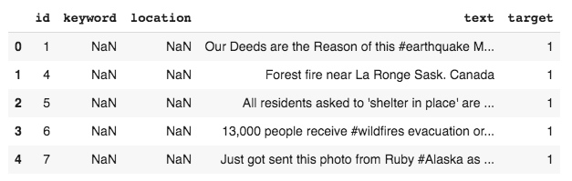
As you can see, the data contains five columns, out of which the text and the target column are required for our model development. You can check the number of datapoints by using the shape command - there are 7613 data points.

07Preprocessing Data

We will first check for the null values in the dataset.

train.isnull().sum()

The output is as follows:

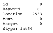
The keyword column has only 61 nulls. To get an idea of what it contains, we plot the distribution of the most common words in this column. Use the following code fragment to plot this distribution:

# empty list for holding keyword from each row of train['keyword']
keyword_combined=[]
for i in range(len(train)):
 keyword_combined.append(train['keyword'].iloc[i])

import collections
# count instances of each keyword
keyword_counters = collections.Counter(keyword_combined)
 
# make dataframe with words and their corresponding counts
keyword_with_counts = pd.DataFrame(keyword_counters.most_common(15),
                            columns=['keyword', 'count'])
 
fig, ax = plt.subplots(figsize=(8, 8))
 
# Plot horizontal bar graph
# plot the frequency distribution after sorting
keyword_with_counts.sort_values(by='count').plot.barh(x='keyword', 
                     y='count',
                     ax=ax,
                     color="purple")
 
ax.set_title("Common Words Found in Tweets")
 
plt.show()

The output is as follows:

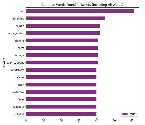
Examining these keywords, we can probably conclude that these won’t be of helpful to us in our model development. Kaggle data description also does not indicate the significance of this column in the model development. So, we will drop this column from our analysis.

As shown in the output of train.isnull().sum(), a large number of records have null value in the location column. As such, this column is not useful for our analysis. So, we will drop it. Also, the column id is not required, as we have a default index in the data frame, provided by Pandas.

We remove all the unwanted columns using the following program statement:

# dropping id, location, keyword column
train.drop(['id','location','keyword'],axis=1,inplace=True)

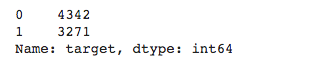
We will now examine how many records in the training dataset are marked as “disaster?”

train['target'].value_counts()

The output is as follows:

08Cleaning Data

Install the clean-text package for cleaning the tweets data. The tweets may contain urls, numbers, etc., which are not useful to us in our model development. The clean-text package allows an easy removal of such items.

!pip install clean-text[gpl] 
from cleantext import clean

We define a function for cleaning an input text with several configurable parameters.

def text_cleaning(text):
text=clean(text,
  fix_unicode=True,               # fix various unicode errors
  to_ascii=True,                 # transliterate to closest ASCII representation
  lower=True,                    # lowercase text
  no_line_breaks=True,           # fully strip line breaks
  no_urls=True,                  # replace all URLs with ''
  no_emails=True,                # replace all email addresses with ''
  no_phone_numbers=True,         # replace all phone numbers with ''
  no_numbers=True,               # replace all numbers with ''
  no_digits=True,                # replace all digits with ''
  no_currency_symbols=True,      # replace all currency symbols with ''
  no_punct=True,                 # fully remove punctuation
  replace_with_url="",
  replace_with_email="",
  replace_with_phone_number="",
  replace_with_number="",
  replace_with_digit="",
  replace_with_currency_symbol="",
  lang="en"                      # set to 'en' for English
)
return text

The clean function has various parameters that help in cleaning the given text in one go. The parameters are mostly self-explanatory. It fixes unicode errors, converts text to ASCII, lowercases the text, and removes line breaks. The clean function also has the ability to trace and replace every occurrence of url, email, phone number, digit and currency symbol with a special symbol, in our case we replace all such occurrences with a space. Set the language parameter as “en” for English.

We now call this function on the entire tweet data.

for i in range(len(train)):
train['text'].iloc[i]=text_cleaning(train['text'].iloc[i])

Next, let’s remove the stopwords from the text. A stop word is a commonly used word (such as “the”, “a”, “an”, “in”) that generally a search engine is programmed to ignore, both while indexing entries and while retrieving them as a result of a search query. As these words do not indicate a disaster or not-a-disaster, we will remove those from our analysis. NLTK (Natural Language Toolkit) in python has a list of stopwords stored in 16 different languages. We will be using this ntlk library to get rid of stopwords in the texts through the code below.

We have to first download ‘stopwords’ from ntlk.

import nltk
from nltk.corpus import stopwords
nltk.download('stopwords')

Select stopwords in English out of the 16 different languages that ntlk supports.

stoplist = stopwords.words('english')

Remove the stopwords from the training data using the following loop:

for i in range(len(train)):
train['text'].iloc[i] = [word for word in train['text'].iloc[i].split() if word not in stoplist]

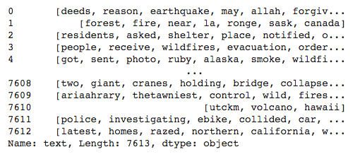
Let’s see our final cleaned text after the stopwords are removed

print(train['text'])

The output is as follows:

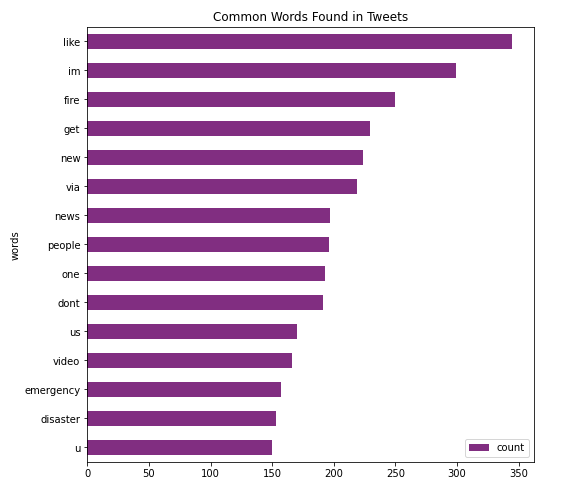
Like the keywords distribution that you checked above, we can examine the distribution of the most common words found in the tweets.

Let’s look at the frequency distribution of unique words in train[‘text’]

# empty list for holding words from each row of train['text']
text_combined=[]

Making a combined list of all the words from each tweet.

for i in range(len(train)):
text_combined.append(train['text'].iloc[i])

Convert the 2-dimensional array of words to 1-dim for easy counting of words.

from itertools import chain
flatten_list_text = list(chain.from_iterable(text_combined))

Count instances of each word using collections.

import collections
word_counters = collections.Counter(flatten_list_text)

Make a dataframe with words and their corresponding counts.

words_with_counts = pd.DataFrame(word_counters.most_common(15), 
columns=['words', 'count'])

We will first sort the words in decreasing order of their instances and then plot the most occurring words using matplotlib.

fig, ax = plt.subplots(figsize=(8, 8))
 
# Plot horizontal bar graph
# plot the frequency distribution after sorting
words_with_counts.sort_values(by='count').plot.barh(x='words', 
                     y='count',
                     ax=ax,
                     color="purple")
 
ax.set_title("Common Words Found in Tweets")
 
plt.show()

The output is as follows:

We will now feed this cleaned-up data to a BERT model for Natural Language Modeling.

09Modeling and Training

We will write our neural network model where the first layer will be the pre-trained BERT model followed by our own network layers.

We write a function as follows for building the model:

def build_model(transformer, max_len=512):
input_word_ids = Input(shape=(max_len,), dtype=tf.int32, name="input_word_ids")
sequence_output = transformer(input_word_ids)[0]
cls_token = sequence_output[:, 0, :]
x = tf.keras.layers.Dropout(0.35)(cls_token)

# make output dense layer
out = Dense(1, activation='sigmoid')(x)

model = Model(inputs=input_word_ids, outputs=out)
model.compile(Adam(lr=3e-5), loss='binary_crossentropy',
              metrics=[tf.keras.metrics.AUC()])

return model

In the above model, the transformer output is passed through a dropout to take care of overfitting, if any. We then pass the output through a dense layer with sigmoid activation. We create a model using the Model function with the appropriate parameter values for inputs and outputs as defined above. We compile the model with Adam optimizer and binary cross entropy loss function.

We use the bert-based-uncased pretrained model and pass it our above written build_model function for constructing our model.

with strategy.scope():
transformer_layer = transformers.TFBertModel.from_pretrained('bert-base-uncased')
model = build_model(transformer_layer, max_len=512)

Print the model summary:

model.summary()

The output is as follows:

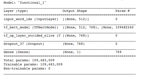
Notice the layers which we added to the output of the BERT layer. Next, we will tokenize the text data for model training.

10Data Preprocessing

We first tokenize all our input datasets - training and testing. You will use the BERT pre-trained tokenizer for this purpose. You create a tokenizer instance using the following statement:

import transformers
tokenizer = transformers.BertTokenizer.from_pretrained('bert-base-uncased')

Save the loaded tokenizer to your local environment.

save_path = 'distilbert_base_uncased/'
if not os.path.exists(save_path):
   os.makedirs(save_path)
tokenizer.save_pretrained(save_path)

Reload it with the Hugging Face tokenizers library.

from tokenizers import BertWordPieceTokenizer
fast_tokenizer = BertWordPieceTokenizer('distilbert_base_uncased/vocab.txt', lowercase=True)
fast_tokenizer

You will be using this fast_tokenizer to encode our input. Next, we write an encode function that uses the above tokenizer for encoding the given text.

def fast_encode(texts, tokenizer, size=256, maxlen=512):
tokenizer.enable_truncation(max_length=maxlen)  # truncate the text and limit it to maxlen
tokenizer.enable_padding(length=maxlen)         # pad sentences shorter than maxlen
ids_full = []

for i in tqdm(range(0, len(texts), size)):
    text = texts[i:i+size].tolist()
    encs = tokenizer.encode_batch(text)        
    ids_full.extend([enc.ids for enc in encs])

return np.array(ids_full)

The fast_encode encodes the text to numbers so that it can be used for model training. Typically, it is used for getting tokens, token types, and attention masks. It outputs a dictionary of encoded text. We now use this encode function to encode our training and testing datasets.

x = fast_encode(train.text.astype(str), fast_tokenizer, maxlen=512)

11Preparing Datasets

We prepare the dataset for training by creating batches of data using

tf.data.Dataset.

BATCH_SIZE=64

y=train['target'].values

We reserve 10% data for testing:

from sklearn.model_selection import train_test_split
X_train, X_test, y_train, y_test = train_test_split(x,y,test_size=0.1, random_state=42)

We create the training dataset using the following statement. The AUTOTUNE parameter prepares the next batch of data while processing the current one.

train_dataset = (
  tf.data.Dataset
    .from_tensor_slices((X_train, y_train))
    .repeat()
    .shuffle(2048)
    .batch(BATCH_SIZE)
  .prefetch(tf.data.experimental.AUTOTUNE)
)

Likewise, we prepare the testing dataset using following code:

test_data = (
  tf.data.Dataset
  .from_tensor_slices(X_test)
  .batch(BATCH_SIZE)
)

12Model Training

We train the model by calling its fit method. The strategy decides on the distribution strategy on the TPU cluster during training.

with strategy.scope():
train_history = model.fit(
  train_dataset,
  steps_per_epoch=150,
  epochs = 10
)

Each epoch took about 43 seconds during my training.

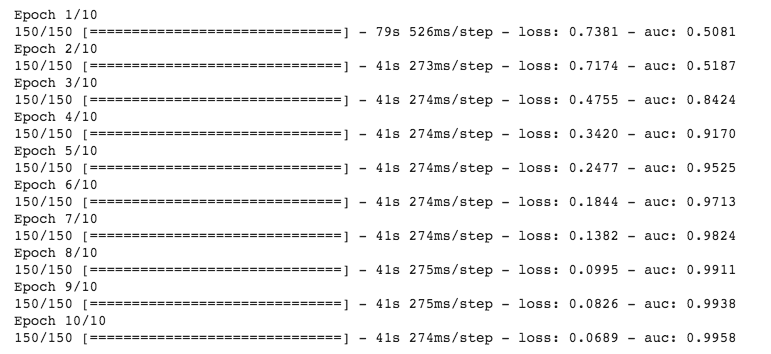
Now, as we have trained and developed the model, it is time to test its inference on the test data.

13Inference on Test Data

We use the predict method to do the inference on the test data.

predictions = model.predict(X_test)

We flatten the predictions from 2-dim to a 1-dimensional array

flattened_predictions = list(chain.from_iterable(predictions))

We convert the predictions to '0' (non-disaster) or '1' (disaster) using a simple if condition

for i in range(len(flattened_predictions)):
if flattened_predictions[i] <= 0.5:
  flattened_predictions[i] = 0
else:
  flattened_predictions[i] = 1

We print the first five predictions:

flattened_predictions[:5]

The output is as follows:

[0, 0, 1, 0, 0]

The output indicates that the third tweet indicates a disaster while the rest indicate non-disaster. You may verify the validity of these predictions by reading out the first five tweets from the test dataset.

Checking out the accuracy with the predictions that we made on X_test and comparing it with y_test.

from sklearn.metrics import accuracy_score
accuracy_score(y_test, flattened_predictions)

This gives accuracy around 79%, which is decent enough for us to continue further. Improving on the accuracy, we may need additional training data and playing around with dropout and a few more network layers.

Now, as we have trained and tested the model, let us try it out on some real-time tweets.

14Analyzing Live Tweets

Twitter provides an API for accessing the live tweets. Install the tweepy Python client for the official Twitter API.

!pip install tweepy

Import the following packages in your project.

import re
import tweepy
from tweepy import OAuthHandler
from cleantext import clean

15Registering with Twitter

To use live tweets in your app, you need to register the app with Twitter. Login into your Twitter account and follow the steps below to register the app.

Open the Login page of Twitter.

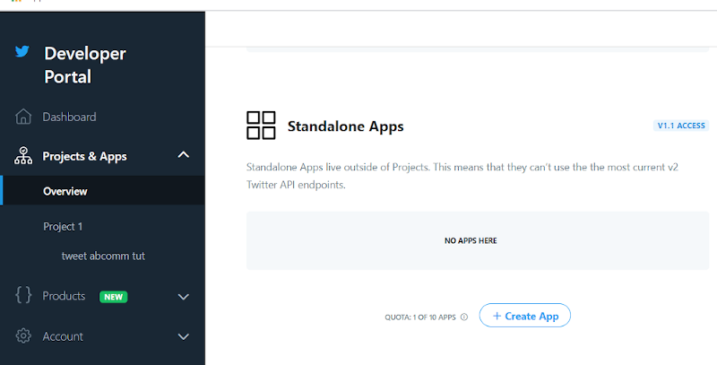
Click the button: ‘Create App’

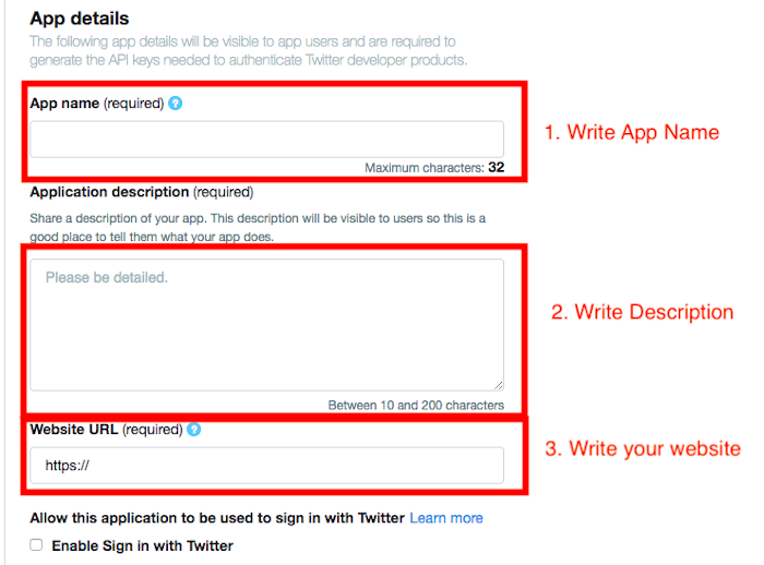
Fill the application details. You may leave the website url field empty. Once the app is created, you will be redirected to the app page.

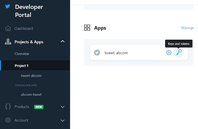
Open the ‘Keys and Access Tokens’ tab.

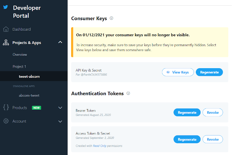
Click the view keys button and your keys will be shown. You might be required to regenerate the access token and secret if you don’t see automatically generated access token and secret.

Copy ‘Consumer Key’, ‘Consumer Secret’, ‘Access token’ and ‘Access Token Secret’.

We will now define a few functions for capturing, preparing and classifying tweets.

16Tokenizing Tweets

Just the way, we tokenize the tweets in our training dataset, we need to tokenize the real-time captured tweets for making predictions on them. The function convert_lines accepts a tweet text as input and tokenizes its contents using the specified tokenizer.

# convert tweet into tokens.   
def convert_lines(tweet, max_seq_length,tokenizer):
 max_seq_length -=2
 all_tokens = []
 
 tokens_a = tokenizer.tokenize(tweet)
 if len(tokens_a)>max_seq_length:
   tokens_a = tokens_a[:max_seq_length]
 
 # remove stopwords
 from nltk.corpus import stopwords
 import nltk
 stoplist = stopwords.words('english')
 tokens_b = [word for word in tokens_a if not word in stoplist]
 
 one_token = tokenizer.convert_tokens_to_ids(["[CLS]"]+tokens_b+["[SEP]"])+[0] * (max_seq_length - len(tokens_b))
 all_tokens.append(one_token)
 
 return np.array(all_tokens)

The above process of tokenizing is exactly the same as what we did for the training dataset.

Then, we write a function for predicting the contents of a given tweet.

def predict_disaster(tweet):
      
maxlen = 512

tweet2 = text_cleaning(tweet)

token_input2 = convert_lines(tweet2,maxlen,tokenizer)

seg_input2 = np.zeros((token_input2.shape[0],maxlen))
mask_input2 = np.ones((token_input2.shape[0],maxlen))

hehe = model.predict([token_input2, seg_input2, mask_input2],verbose=1,batch_size=32)

if hehe <= 0.5:
  return 'no disaster'
else:
  return 'real disaster'

The function uses our pre-trained model and returns its prediction as a boolean value - disaster or non-disaster.

Lastly, we develop one more function for capturing live tweets from Twitter using our previously created tokens and keys. The function returns the original tweets that we load along with their class prediction that we get from the above written predict_disaster function. The function load_tweets is created as follows:

def load_tweets(query, consumer_key, consumer_secret, access_token, access_token_secret,count = 10):
      
# attempt authentication
try:
   # create OAuthHandler object
   auth_handle = OAuthHandler(consumer_key, consumer_secret)
 
   # set access token and secret
   auth_handle.set_access_token(access_token, access_token_secret)
  
   # create tweepy API object to fetch tweets
   api = tweepy.API(auth_handle)

except:
   print("Error: Authentication Failed")

# empty list to store parsed tweets
tweets = []
try:
   # call twitter api to fetch tweets
   our_tweets  = api.search(q = query, count = count)
    # parsing tweets one by one
   for tweet in our_tweets :

       # empty dictionary to store required params of a tweet
       parsed_tweet = {}

       # saving text of tweet
       parsed_tweet['text'] = tweet.text
      
       # saving sentiment of tweet
       parsed_tweet['class'] = predict_disaster(tweet.text)
        # appending parsed tweet to tweets list
       if tweet.retweet_count > 0:
           # if tweet has retweets, ensure that it is appended only once
           if parsed_tweet not in tweets:
               tweets.append(parsed_tweet)
       else:
           tweets.append(parsed_tweet)
    # return parsed tweets
   return tweets
except tweepy.TweepError as e:
   # print error (if any)
   print("Error : " + str(e))

We will now put the whole development into the practice.

17Putting into Practice

Set your keys and tokens from the Twitter Dev Console into the following variables:

consumer_key = 'YOUR CONSUMER_KEY'
consumer_secret = 'YOUR CONSUMER_SECRET'
access_token = 'YOUR ACCESS_TOKEN'
access_token_secret = 'YOUR ACCESS_TOKEN_SECRET'

Input any query and tweets regarding it would come up when the load_tweets function is called with your keys and tokens.

tweets = load_tweets('crime', consumer_key, consumer_secret, access_token, access_token_secret, 200)

Now that the tweets are fully loaded and classified, we would like to see some results.

Let's distribute the tweets in two variables according to their classes and find out Real Disaster tweets percentage and No Disaster tweets percentage.

real_d  = [tweet for tweet in tweets if tweet['class'] == 'real disaster'] 
print("Real Disaster tweets percentage: {} %".format(round((100*len(real_d )/len(tweets)),2)))
 
no_d = [tweet for tweet in tweets if tweet['class'] == 'no disaster']
print("No Disaster tweets percentage: {} %".format(round((100*len(no_d)/len(tweets)),2)))

The output is as follows:

real_d  = [tweet for tweet in tweets if tweet['class'] == 'real disaster'] 
print("Real Disaster tweets percentage: {} %".format(round((100*len(real_d )/len(tweets)),2)))
 
no_d = [tweet for tweet in tweets if tweet['class'] == 'no disaster']
print("No Disaster tweets percentage: {} %".format(round((100*len(no_d)/len(tweets)),2)))

Print first five positive tweets using the following code

print("

 Real Disaster tweets:")
for tweet in real_d[:10]:
   print(tweet['text'])

Print first five negative tweets using the following code

print("

 No Disaster tweets:")
for tweet in no_d[:10]:
   print(tweet['text'])

The output is as follows

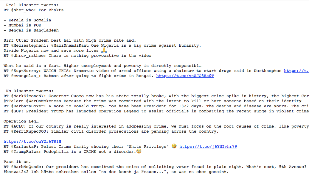
So, this concludes our creation of a Live Tweet Sentiment Classifier. Hope you liked it!

You may also like to look up our earlier tutorial - Detecting Slang Using BERT for a BERT Transfer Learning model.

Stay tuned for more such interesting projects in Deep Learning.

18Summary:

In this tutorial, you learned how to extract live tweets using Twitter API and classify them as disastrous or non-disastrous using Natural Language Processing and BERT Transformer model that has revolutionized solving NLP tasks. The twitter data is usually highly erratic, you learned how to pre-process and clean this data for model training. You learned how to tokenize the text data with BERT fast tokenizer and use the BERT pre-trained model for Natural Language Modeling. You added your own neural network layers to the pre-trained BERT network layer to define your own model for text classification. You learned how to use TPU for distributed training. Then, you learned how to register yourself as a developer on Twitter. You used the Twitter provided tokens and keys for loading the live stream of tweets. You learned how to apply your trained ML model on these tweets to classify them into two categories.